Step-by-Step Guide: Creating a Dropdown Menu From an Excel Cell

Quick Links

• What is an Excel Drop-Down List?
• How to Add a Drop-Down List to Excel

Key Takeaways

• Drop-down lists in Excel make data entry easier and more efficient by allowing users to select pre-determined values from a list of options.
• To add a drop-down list in Excel, use the Data Validation feature and name the range of cells containing the options. Then, enter the name of the cell range in the Source box of the Data Validation dialog box.
• You can customize the behavior of the drop-down list by checking or unchecking options like “Ignore blank” or adding an input message. To remove the drop-down list, open the Data Validation dialog box and click the “Clear All” button.

Drop-down lists are very useful data entry tools we see just about everywhere, and you can add custom drop-down lists to your own Excel worksheets. It’s easy and we’ll show you how.

What is an Excel Drop-Down List?

A drop-down list in Excel is exactly like any other drop-down list you’re familiar with — just click the arrow then select one of a few pre-determined values. Drop-down lists make it easier and more efficient to enter data into your spreadsheets.

You can add drop-down lists to cells in Excel containing options such as “Yes” and “No”, “Male” and “Female,” or any other custom list of options, including numbers or special characters.

How to Add a Drop-Down List to Excel

Drop-down lists are created using the Data Validation feature in Excel — not particularly intuitive. We’re going to create a drop-down list with a selection of age ranges to show you an example. We created three labeled columns : Name, Age, and Sex, and filled in two example names. You can do as many or as few as you like.

To begin, enter the list of age ranges into sequential cells down a column or across a row. We entered our age ranges into cells A7 through A11 on the same worksheet, as shown below. You can also add your list of options to a different worksheet in the same workbook.

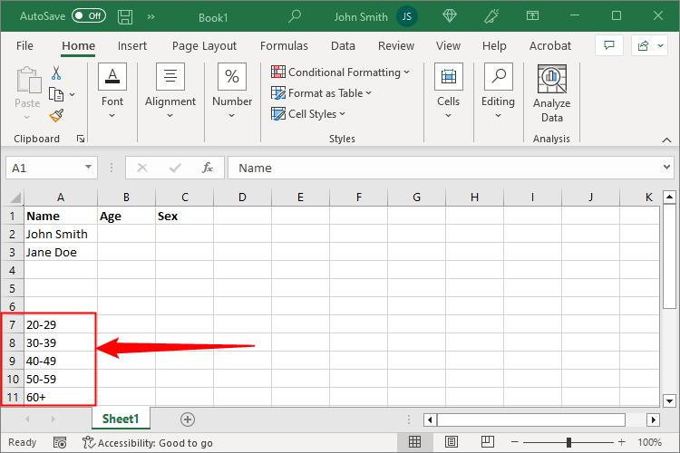
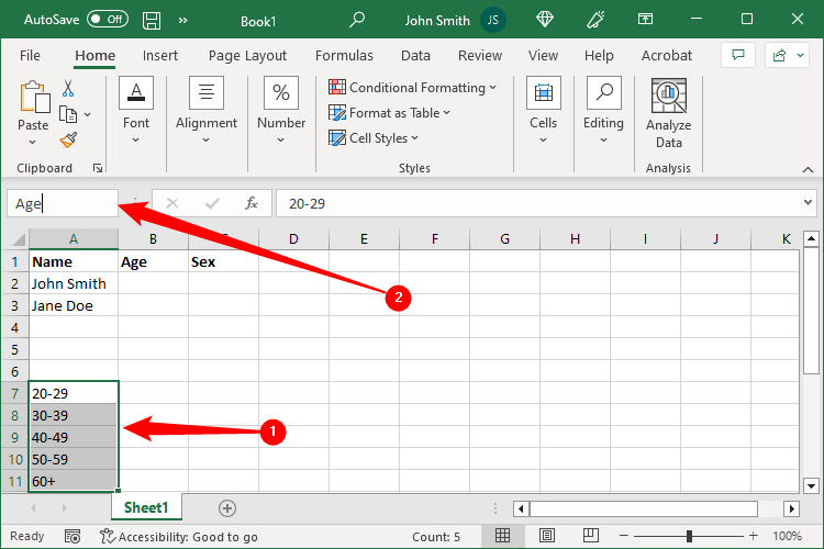
Now, we’re going to name our range of cells to make it easier to add them to the drop-down list. To do this, select all the cells containing the drop-down list items and then enter a name for the cell range into the Name box above the grid. We named our cell range Age.

Hold Ctrl while you click to select multiple cells in Excel on Windows. On a Mac, hold Command and click to select multiple items. You can also hold Shift-click the first cell and then Shift-click the last cell to select all of the cells in between as well.

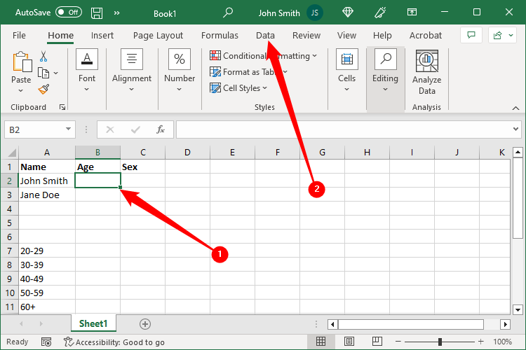
Now, select the cell into which you want to add a drop-down list and click the “Data” tab.

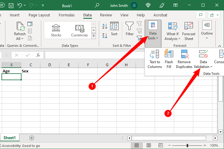
Open the Data Tools section of the Data tab, then click the “Data Validation” button

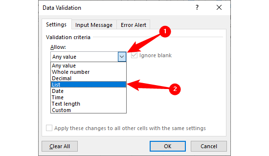
The Data Validation dialog box displays. On the Settings tab, select “List” from the Allow drop-down list (see, drop-down lists are everywhere!).

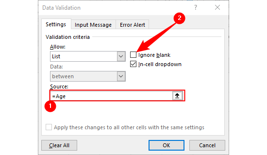
Now, we’re going to use the name we assigned to the range of cells containing the options for our drop-down list. Enter =Age in the “Source” box (if you named your cell range something else, replace “Age” with that name). Make sure the “In-cell dropdown” box is checked.

The “Ignore blank” check box is checked by default. This means that the user can select the cell and then deselect the cell without selecting an item. If you want to require the user to select an option from the drop-down list, uncheck the Ignore blank check box.

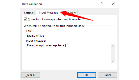
You can add a popup message that displays when the cell containing the drop-down list is selected. To do this, click the “Input Message” tab on the Data Validation dialog box. Make sure the “Show input message when the cell is selected” box is checked. Enter a Title and an Input message and then click the “OK” button.

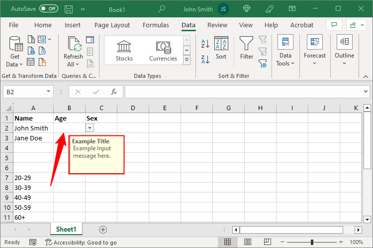
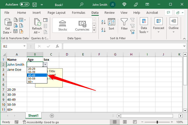
When the cell containing the drop-down list is selected, you’ll see a down arrow button to the right of the cell. If you added an input message, it displays below the cell. The down arrow button only displays when the cell is selected.

Click the down arrow button to drop down the list of options and select one.

Of course, we have an entire column we want to take age values. There are a few ways to make that happen. The first — and easiest — is just to select all of the cells you want to have a drop-down menu before you go to Data Validation and actually add the drop-down menu. The simplest way to select every cell in a column is to click the column header. If you have a cell you’re using for a label, just Ctrl+Click it to deselect it, so the formatting doesn’t get applied there.

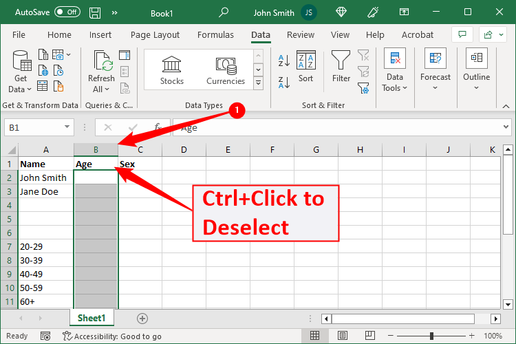
Then just apply the formatting just like we showed you previously.

The other scenario is when you’ve already applied the drop-down menu formatting to one cell, but don’t want to have to repeat the process of creating a drop-down menu. In this case, just click and select the cell that already has the drop-down menu. Note the small square in the bottom-right corner of the cell. Left-Click and drag that corner down to all of the cells you want to have a drop-down menu, then release your mouse. The cells you dragged to will have inherited the drop-down menu from the original cell. It’ll look like this:

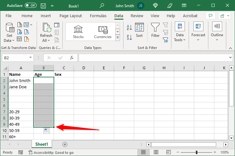
This trick basically applies to any formatting you apply to a cell in Excel, not just drop-down menus.

If you decide you want to remove the drop-down list from the cell, open the Data Validation dialog box as described earlier and click the “Clear All” button, which is available no matter which tab is selected on the dialog box.

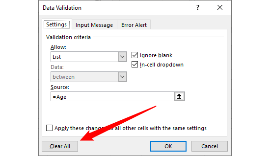
The options on the Data Validation dialog box are reset to their defaults. Click “OK” to remove the drop-down list and restore the cell to its default format.

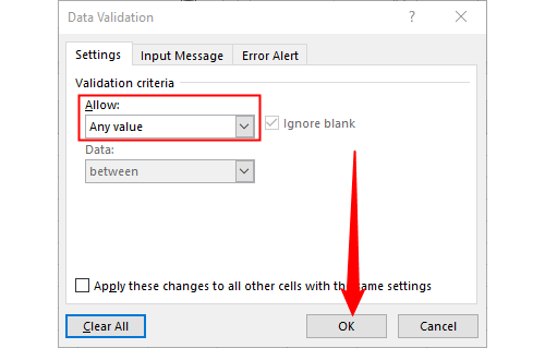
If there was an option selected when you removed the drop-down list, the cell is populated with the value of that option.

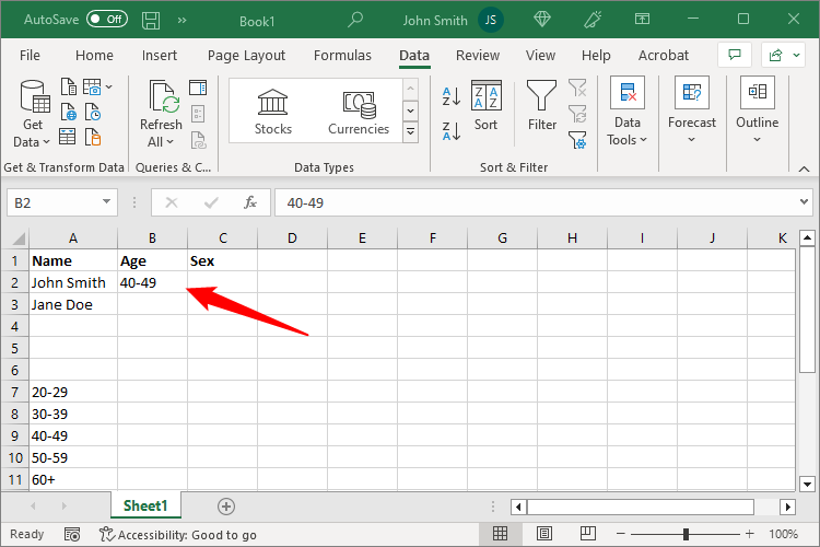
Follow this process to add drop-down lists to other cells as needed. You can use the same list for multiple drop-down lists. If you have many drop-down lists you need to add on a worksheet, you may want to put the lists of options on another worksheet in the same workbook. You can hide the worksheet containing your lists of options to prevent them from being changed.

Also read: