Mastering Text Editing in Excel: Discover These 9 Powerful Features

Quick Links

Functions in Excel aren’t just for numbers and calculations. You can use functions when working with text too. Here are several helpful Microsoft Excel text functions.

Whether you want to change the letter case, find text within another string, substitute old text with something new, or combine text from multiple cells, there’s a function here for you.

Convert the Letter Case: UPPER, LOWER, and PROPER

You may want your text to contain all uppercase or all lowercase letters. Or maybe you want the first letter of each word capitalized. This is when the UPPER, LOWER, and PROPER functions come in handy.

The syntax for each is the same with just one required argument:

UPPER(cell_reference)
LOWER(cell_reference)
PROPER(cell_reference)

To change the text in cell B4 to all uppercase letters, use the following formula:

=UPPER(B4)

To change the text in that same cell to all lowercase letters, use this formula instead:

=LOWER(B4)

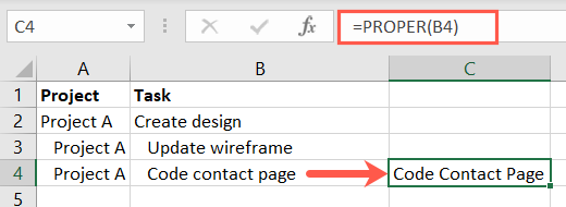
To change the text in cell B4 to capitalize the first letter of each word, use this formula:

=PROPER(B4)

Remove Spaces: TRIM

You may have extra spaces in the text that you want to remove. The TRIM function takes care of eliminating spaces without manual work.

The syntax for the function is TRIM(text) where you can enter the text in quotes or use a cell reference in the formula.

To remove the spaces in the phrase “ trim spaces “ you would use the following formula:

=TRIM(“ trim spaces “)

To remove the spaces in the text in cell A1, you would use the cell reference as in this formula:

=TRIM(A1)

Compare Text Strings: EXACT

Maybe you have two cells containing text that you want to compare and see if they match exactly . Appropriately named, the EXACT function comes to the rescue.

The syntax for the function is EXACT(cell_reference1, cell_reference2) where both cell references are required. The result is True for an exact match or False for no match.

To compare the text in cells A1 and B1, you would enter the following formula:

=EXACT(A1,B1)

In this first example, the result is True. Both text strings are identical.

In the second example, the result is False. The text in cell A1 has uppercase letters whereas the text in cell B1 does not.

In our final example, the result is False once more. The text in cell B1 has spaces that the text in cell A1 does not.

Locate Text Within a String: FIND

If you want to find specific text within another string of text, you can use the FIND function. Keep in mind that the function is case-sensitive and does not use wildcards.

The syntax for the function is FIND(find, within, start_number) where the first two arguments are required. The start_number argument is optional and allows you to specify with which character position to start the search.

To find “QR1” within the text in cell A1, you would use this formula:

=FIND(“QR1”,A1)

The result shown below is 8 representing the eighth character in the string as the start of the located text.

To find the letter F in cell A1 beginning with the fourth character, you would use this formula:

=FIND(“F”,A1,4)

The result here is 6 because that is the character position for first capital F after the fourth character.

Replace Existing Text Using a Position: REPLACE

If you’ve ever had to replace text based on where it exists in a text string, you’ll appreciate the REPLACE function.

The syntax for the function is REPLACE(current_text, start_number, number_characters, new_text) where each argument is required. Let’s look at the details for the arguments.

Current_text: The cell reference(s) for the current text.
Start_number: The first character’s numeric position in the current text.
Number_characters: The number of characters you want to replace.
New_text: The new text to replace the current text.

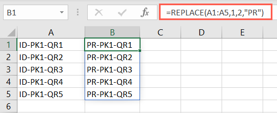
In this example, the first two characters of our product IDs in cells A1 through A5 are changing from “ID” to “PR.” This formula would make that change in one fell swoop:

=REPLACE(A1:A5,1,2,”PR”)

To break that down, A1:A5 is our cell range, 1 is the position of the first character to replace, 2 is the number of characters to replace, and “PR” is the new text.

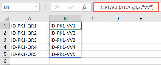
Here’s another example for that product ID. Using this formula, we can change the eighth and ninth characters in the string “QR” with “VV.”

=REPLACE(A1:A5,8,2,”VV”)

To break this one down, A1:A5 is our cell range, 8 is the position of the first character to replace, 2 is the number of characters to replace, and VV is the new text.

Substitute Current With New Text: SUBSTITUTE

Similar to REPLACE, you can use the SUBSTITUTE function to change the actual text rather than using a character’s position.

The syntax is SUBSTITUTE(cell_reference, current_text, new_text, instances) where all arguments are required except for instances. You can use instances to specify which occurrence in the text string to change.

To change the last name Smith to Jones in cell A1, use the following formula:

=SUBSTITUTE(A1,”Smith”,”Jones”)

To change “Location 1, Quarter 1” to “Location 1, Quarter 2” in cell A1, you would use this formula:

=SUBSTITUTE(A1,”1”,”2”,2)

Breaking down this formula, A1 is the cell reference, 1 is the current text, 2 is the new text, and the final number 2 is the second instance in the string. This ensures that only the second occurrence of the number 1 is changed.

Combine Text: CONCAT

One final function you may find helpful when working with text is CONCAT. This function helps you join text from multiple strings or locations into one string, or add to currently existing text .

The syntax for the function is CONCAT(text1, text2) where only the first argument is required, but you’ll likely always use the second argument.

To join the text in cells A1 and B1 with a space between the words, use this formula:

=CONCAT(A1,” “,B1)

Notice that the quotes contain the space to add.

To join that same text but add the prefix Mr. and a space in front, you would use this formula:

=CONCAT(“Mr. “,A1,” “,B1)

Here you have Mr. with a space in the first set of quotes, the first cell reference, another space within quotes, and the second cell reference.

Hopefully these Excel text functions help you manipulate your text in less time and with less effort.

Win Forum

Mastering Text Editing in Excel: Discover These 9 Powerful Features