Mastering Differences: A Step-by-Step Guide to Comparing Excel Lists

Quick Links

Microsoft Excel offers two different methods to help you compare two lists and highlight the missing items in each one. You can choose to highlight the missing items in both lists or in a single one. We’ll show you how.

The Quick Way: Highlight Unique Cells to Compare Lists

A quick way to compare two lists in your spreadsheet is to use Excel’s unique highlight feature . This feature highlights the items in a list that are not found in the other list. This way you know exactly what items are missing from your lists.

To use the method, first, select the lists you want to compare in your spreadsheet.

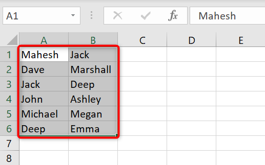
While your lists are highlighted, in Excel’s ribbon at the top, click the “Home” tab.

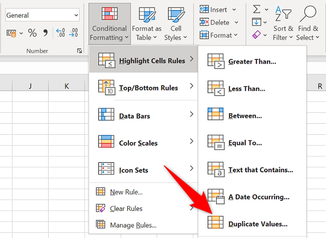
On the “Home” tab, in the “Styles” section, click Conditional Formatting > Highlight Cells Rules > Duplicate Values.

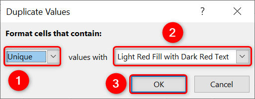
In the “Duplicate Values” box, click “Duplicate” and choose “Unique.” Click the second drop-down menu and choose how you would like to highlight the missing items. To specify your own formatting, choose “Custom Format” from the menu.

Then apply your changes to your lists by clicking “OK.”

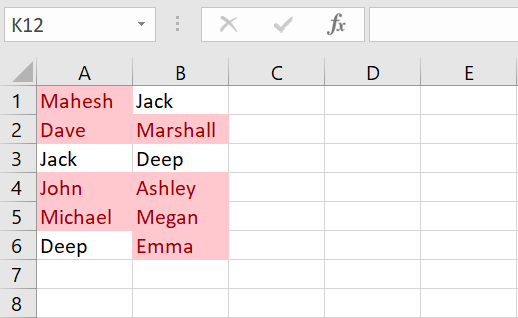
Excel will highlight the missing items in your lists. For example, in your first list, you will have those items highlighted that are missing from the second list, and so on.

And that’s it.

The Formula Way: Use Conditional Formatting to Compare Lists

The above method highlights items in both your lists. If you’d only like to highlight missing items in a specific list, then use a formula with conditional formatting as explained below.

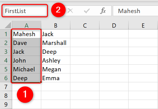
First, in your spreadsheet, select all rows of your first list. Then, in the top-left corner, click the text box, type

    `FirstList`

, and press Enter. This assigns a unique name to your range of cells , which lets you refer to all these cells using a single name.

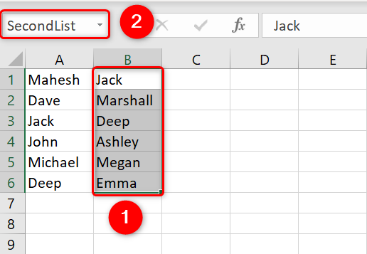
Assign a unique name to your second list by first selecting all rows of your list. Then, in the top-left corner, click the text box, type

    `SecondList`

, and press Enter.

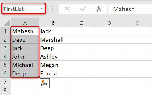
Select all rows of your first list by clicking the text box in the top-left corner and choosing “FirstList.”

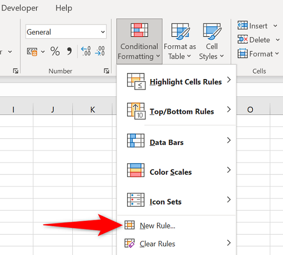
In Excel’s ribbon at the top , click the “Home” tab and choose Conditional Formatting > New Rule.

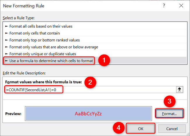
On the “New Formatting Rule” window, you’ll specify how your missing items will be highlighted. On this window, from the “Select a Rule Type” section, choose “Use a Formula to Determine Which Cells to Format.”

In the “Format Values Where This Formula is True” box, type the following:

=COUNTIF(SecondList,A1)=0

Select the “Format” button and specify how you’d like to format the missing items in your list. Then, save your changes by clicking “OK.”

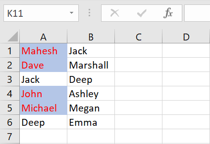
Back on the spreadsheet, Excel has highlighted the items in your first list that are missing from the second list. Your job is done.

And that’s how you quickly perform a comparison of two different lists in your Excel spreadsheets. Very useful!

You can also alphabetize your data to manually find the differences in two lists in your spreadsheets. Check out our guide to learn how to do that.

Win Forum

Mastering Differences: A Step-by-Step Guide to Comparing Excel Lists