Mastering, Advanced, Sophisticated, and Unlocking.

Quick Links

Key Takeaways

To create an advanced filter in Excel, start by setting up your criteria range. Then, select your data set and open the Advanced filter on the Data tab. Complete the fields, click OK, and see your data a new way.

While Microsoft Excel offers a built-in feature for filtering data , you may have a large number of items in your sheet or need a more complex filter. Here, we’ll explain how to create an advanced filter in Excel.

How to Set Up the Criteria Range

Before you can use the advanced filter in Excel, you’ll need to create a cell range for the conditions you’ll use.

Add at least a few rows above your data to get started; you can always insert more rows if needed. Keep in mind, you’ll need one row for the labels and one empty row between the criteria and the data.

In the top row, enter your columns labels. These should match those for your data as they’ll be used for the filter criteria.

We’ll be using an example throughout this tutorial, so below is the data we’re using.

Click here

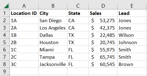
We then insert five rows above our data. We have one row for labels, three for criteria, and one blank row. We then copy our column headers into the first row. So, now our sheet looks like this:

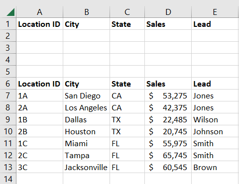
Once you have the range for your filter conditions set up, you’re ready to create the advanced filter.

You can name your criteria range to automatically pop it into the filter if you like.

Entering Criteria for an Advanced Filter in Excel

To enter criteria for your advanced Excel filter into a cell, you’ll use the format

    `="=variable"`

The first equal sign begins the string and the quotations marks contain the criteria. You can use the normal comparison operators for your conditions. Here are a few examples.

Equal to Smith:
="=Smith"
Not equal to Smith:
="<>Smith"
Less than 100:
="<100"
Greater than or equal to 100:
=">=100"

When you type the criteria this way into the cell, Excel converts it to the format it needs for the filter.

How to Use a Single Criterion, Single Column Excel Filter

The best way to get started is with a simple example using one condition and one column. Here, we’ll filter our data based on the Location ID 2B.

Go to the Location ID column and enter the following for equals 2B into the first row below the label:

=”=2B”

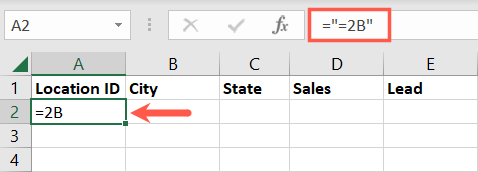
Next, select a cell in your data set, head to the Data tab, and pick “Advanced” in the Sort & Filter section of the ribbon.

In the pop-up box, start by choosing where you want the filtered data to appear. You can filter it in place or in another location. If you choose the latter, enter the location in the Copy To box.

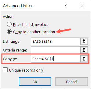
Now confirm the cells in the List Range box. Excel should have added them for you automatically, so simply make sure they’re correct.

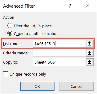
Then, enter the cell range into the Criteria Range box. You can do this easily by clicking inside the box and then using your cursor to drag through the range in your sheet. Be sure to include the column label cells and only additional rows with cells that contain criteria. If you include empty rows , it’s highly likely that your filter results will be incorrect.

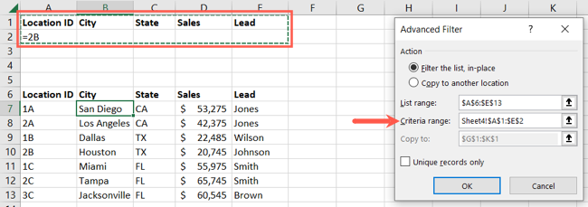
Optionally check the box if you want unique records only. Click “OK” when you finish.

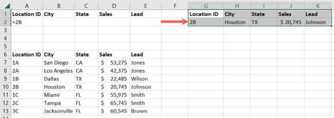
You should then see your filtered data. If you chose to filter your data in place, the other rows should be hidden. Here, we picked a location in our sheet for the filtered data.

How to Use a Multiple Criteria, Single Column Excel Filter

Maybe you want to filter data using multiple conditions that appear in a single column. You can do that with an advanced Excel filter. As an example, we’ll filter our data for Location ID’s 1B and 2B.

Go to the Location ID column and enter the criteria in two separate rows, 2 and 3, starting directly below the label.

=”=1B”

=”=2B”

It should look like this:

Select a cell in your data set, go to the Data tab, and pick “Advanced” to open the filter tool.

Complete the same details as before, but this time, expand the criteria range to include the additional condition. Click “OK” to apply the filter.

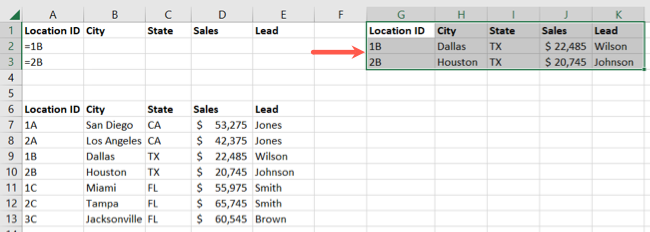
You should then see both results from the filter in the location you chose.

How to Use a Multiple Criteria, Multiple Column Excel Filter

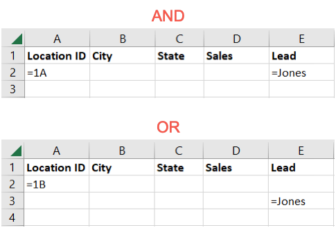
Next, we’ll look at using multiple conditions in an advanced Excel filter. This can be AND or OR criteria. For example, you can filter for Location ID equals 1A and Lead equals Jones where all conditions are true. Or you can filter for Location ID equals 1B or Lead equals Jones where any conditions are true.

All Conditions True

To filter with an AND condition, you’ll place both criteria in the same row below their corresponding labels.

So, we enter the following below the Location ID label in row 2:

=”=1A”

Then, we enter the following below the Lead label, also in row 2:

=”=Jones”

It looks like this:

And just like before, select a cell in the data set, go to the Data tab, and pick “Advanced” to open the tool.

For this filter, we change our criteria range since it only includes rows 1 and 2. Adjust the other options as necessary and click “OK.”

Notice in the screenshot that Excel has named our criteria range for us. You may see the same thing when reusing the same cell range.

We then have our one result. Remember that placing the criteria in the same row indicates the AND operator. So, even though we have Jones as a Lead for two locations, we filtered for only location 1A with Jones.

Any Conditions True

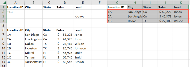
Next, we’ll filter by multiple conditions again, but using OR criteria. For this, you place the conditions in separate rows below the corresponding labels.

So, we enter the following below the Location ID label in row 2:

=”=1B”

Then, we enter the following below the Lead label, but in row 3:

=”=Jones”

It looks like this:

Open the Advanced filter tool as before, adjust the criteria range to accommodate the additional row, and click “OK.”

As you can see, we have three results, one for 1B and two for Jones. Because we used the OR criteria, any conditions we included were met.

The key to setting up a multiple criteria filter in Excel is that for AND criteria, you place the conditions in the same row and for OR criteria, you place the conditions in separate rows.

Any and All Conditions True

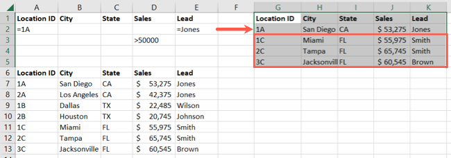
For one final example, we’ll apply a more complex filter using AND and OR criteria together with a different comparison operator. We’ll filter for Location ID equals 1A and Lead equals Jones or Sales is greater than 50,000.

In row 2, we enter the following criteria below Location ID and Lead respectively:

=”=1A”

=”=Jones”

In row 3, we enter the next condition below the Sales label:

=”>50000”

This setup looks like this:

Open the Advanced filter tool, double-check or adjust the fields as needed, and click “OK.”

You’ll then see the results. Here, we have row 2 containing our AND criteria, 1A and Jones. Then, additional rows 3 through 5 containing our OR criteria for Sales greater than 50,000.

If you have a large amount of data in your spreadsheet and need a more robust filter option , keep the advanced filter in Excel in mind.

Win Forum

Mastering, Advanced, Sophisticated, and Unlocking.